The Identification of Distinct Midfielder Archetypes in Modern Football
UNSUPERVISED LEARNING · PLAYER PROFILING
Traditional football analysis often classifies midfielders into three generic roles: central midfielders (CMs), defensive midfielders (DMs) and attacking midfielders (AMs). However, modern tactical systems have blurred these lines and created far more fluid roles. This project uses unsupervised learning techniques to identify distinct midfielder archetypes based on performance metrics, providing a more nuanced understanding of player roles in modern football.
Methodology
01. Data Collection and Preprocessing
The dataset, taken from the 2024/25 season, contains a 456 midfielders playing in Europe's top five leagues. It contains a range of defensive, creative and possession-based metrics, expressed in raw, per 90 and success-rate formats, alongside basic player information such as position, nationality, and preferred foot.
This analysis primarily used per 90 stats to standardise player performance across differing playing times. However, per 90 stats are unreliable with small sample sizes. For example a player who plays 45 minutes and scores once will have a misleading rate of 2 goals per 90 stat of 2. Therefore, all players who played fewer than 900 minutes (10 full games) across the season were removed from the data set to reduce noise and improve staistical reliability.
02. Feature Engineering
Of the original 88 metrics in the dataset, 22 were selected and grouped together into five categories that are important to describe the profile of midfielders:
- Progression - Progressive Passes per 90, Passes Into the Penalty Area per 90, Progressive Runs per 90 and Dribbles per 90.
- Creativity - Expected Assists per 90, Key Passes per 90, Shot Assists per 90 and Smart Passes per 90.
- Defensive Contributions - Defensive Duels Won (%), Ariel Duels Won (%), Possession Adjusted Interceptions per 90 and Successful Defensive Actions per 90.
- Goal Scoring Threat - Non-Penalty Goals per 90, Expected Goals per 90, Shots per 90 and Touches in the Box per 90.
- Possession Involvement - Passes per 90, Accurate Short / Medium Passes per 90, Recieved Passes per 90, Successful Passes per 90, Back Passes per 90 and Lateral Passes per 90.
Both per 90 stats as well as percentage stats were used, to measure both involvement and efficinecy, providing a more reliable player profile.
03. Z-Score Standardisation
Before combining the metrics within each category, all features were standardised using Z-scores. This was a necessary step because raw football metrics exist on different scales, e.g. shots per 90 may be 3.4 while xG per 90 may be 0.08. Without scaling, high-magnitude metrics would dominate the aggregated scores.
Z-scores transform each statistic by measuring how far a player's performance is from the dataset mean in units of standard deviation. A value of 0 represents a perfectly average performance, while positive and negative scores indicate above and below-average perforamnce respectively.
After standaradisation, the mean of all z-scores within each category is calculated to produce a single score, representing a player's performance within that category.
04. Dimensionality Reduction
After feature engineering, each player is represented by five scores, one for each category. However, it is impossible to visualise the relationship between these in all five dimensions. To address this, dimensionality reduction techniques were used to reduce the data into two dimensions. Dimensionality reduction achieves this by reducing complexity, while preserving the underlying structure of the data. This means players that are statistically similar across the five categories should remain close together in the reduced two-dimensional space. To ensure the robustness of the results, three different dimensionality reduction techniques were used: Principal Component Analysis (PCA), t-distributed Stochastic Neighbour Embedding (t-SNE) and Uniform Manifold Approximation and Projection (UMAP).
05. Clustering
After dimensionality reduction, the next step was to identify clusters of players with similar profiles. Clustering is an unsupervised learning technique that groups data points based on their similarity. The K-Means clustering algorithm was used, which partitions the data into K distinct clusters by minimizing the variance within each cluster. The key challenge was determining the optimal number of clusters, which was determined using the Elbow Method and Silhouette Analysis, ensuring that the identified clusters were both meaningful and well-separated.
06. Cluster Interpretation
After clustering, the final step was to interpret the characteristics of each cluster. This involved analysing the average scores across the five categories for each cluster, allowing for the identification of distinct midfielder archetypes. By examining these profiles, it was possible to understand the unique roles and contributions of different types of midfielders in modern football.
Dimensionality Reduction
Dimensionality reduction techniques were required to visualise the relationship between the five player categories in two-dimensional space. For the robustness of the analysis, three different techniques were trialied: Principal Component Analysis (PCA), t-distributed Stochastic Neighbour Embedding (t-SNE) and Uniform Manifold Approximation and Projection (UMAP). By comparing the effectiveness of these techniques in reducing complexity while preserving structure, we were ale to identify the most suitable method for visualising the structure of midfielder archetypes in modern football.
Principal Component Analysis (PCA)
PCA is a linear method that projects the data onto directions of maximum variance. It serves as a simple and interpretable baseline but may fail to capture more complex, non-linear relationships between player attributes. To aid the interpretation of the PCA embedding, players are coloured according to their possession score. This demonstrates how PCA reduction works, projecting data onto directions of maximum variation, as seen by the clear gardient along the PC2 axis from bottom to top. This was the result when PCA was applied to the midfielder dataset:
Loading values explain what combination of the original cateogries contribute to the axes values PC1 and PC2 (principal components). We can interpret these components:
- PC1: The strong positives loading values are creativity (0.63), progression (0.50) and goal threat (0.46), while the defensive loading score is negative (-0.27). So we can interpret PC1 as attacking involvement v defensive contribution. Players with a high PC1 score are creative players who are more involved in attacking sequences. While players with a low PC1 score are more defensive and less involved in possession.
- PC2: The only strong positive loading score is possession (0.70), while the dominating negative is goal threat (-0.64). So we can interpret PC2 as direct goal threats v posssession-based controllers. Players with a lower PC2 score are less involved in possession and can be described as box threats, with a good goal scoring ability. Whereas, players with a higher PC2 score are much slower in possession, the midfielder controllers who dictate the tempo of the game.
Also we identified the variance explained by the two principal components. PC1 explains 47% of the variance and PC2 explains 25%, a total of 72%. So, nearly three quarters of the structure in five-dimensional space is presereved when compressed into two-dimensions. This suggests that the engineered category scores provide a compact and informative representation of player performance, suitable for visualisation and further analysis.
t-distributed Stochastic Neighbour Embedding (t-SNE)
t-SNE is a non-linear technique that focuses on preserving local relationships, often producing well-defined clusters of similar players. However, it can distort global structure and is sensitive to parameter choices.
t-SNE relies on one key hyperperameter, Perplexity, which controls the size of the local neighbourhood that each point considers when constructing the embedding. Lower perplexity focuses on very local structure and can lead to fragmented clusters, while high perplexity looks at global structure and might over-smooth the data.
To decide which value of perplexity was best, embeddings were generated for four values (5,15,25,50). The quality of each embedding was evaluated by measuring neighbourhood presevation, defined as the overlap between the k-nearest neighbours in the original 5-D space and the embbedded 2-D space, for which k = 10. These were the results:
The results show that perplexities in the range 15-25 achieve the highest neighbourhood preservation (~ 57%), indicating the best balance between capturing local structure while maintaining global stability. The small variation in values suggests that the embedding is reasonably robust to the choice of perplexity, with 25 selected for future analysis.
To aid interpretation, the t-SNE embedding is coloured according to the possession score. Unlike the PCA projection, no clear global gradient is observed. This reflects the ability of t-SNE to preserve local relationships, where players with similar overall profiles may still differ in specific attributes such as possession behaviour.
Uniform Manifold Approximation and Projection (UMAP)
UMAP is another non-linear method that balances preservation of both local and global structure. It is generally faster and more stable than t-SNE, and is well-suited for uncovering both clusters and continuous gradients in player styles.
UMAP relies on two key hyperperameters, minimum distance and nearest neighbours. The minimum distance controls how tightly similar players are clustered in the embedded space. Lower values pack similar players closer together while higher values spread players out to emphasise broarder variation between clusters. The nearest neighbours value controls how many nearby players are considers when builiding the structure. Lower values prioritise local structure, creating more fragmeneted clusters of highly specific micro roles. Whereas, higher values incorporate more global structure, resulting in smoother embeddings where clusters are more connected but less sharply separated.
To identify a stable configuration of these parameters, we evaluated combinations of:
- Minimum distance: 0.01, 0.1, 0.5
- Nearest neighbours: 5, 15, 30
This resulted in the following nine different UMAP embeddings:
The performance of each configuration was evaluated using two metrics:
- Neighbourhood overlap, measuring how well nearest neighbours in the original feature space are preserved in the embedding.
- Trustworthiness, a more robust metric that quantifies how well local neighbourhood structure is preserved during dimensionality reduction.
Two UMAP configurations achieve near-identical performance in terms of neighbourhood preservation and trustworthiness:
- Minimum distance = 0.01, Nearest neighbours = 15 (overlap = 0.541, trust = 0.954)
- Minimum distance = 0.1, Nearest neighbours = 5 (overlap = 0.534, trust = 0.959)
The differences between these configurations are minimal, suggesting a stable region of the parameter space where UMAP consistently preserves local structure. This indicates that the embedding is robust to small variations in hyperparameters within this range, and no single configuration is clearly superior based on quantitative metrics alone.
For subsequent analysis, we select min_dist = 0.01 and n_neighbors = 15 as the final configuration, as it provides a slightly more structured and visually interpretable clustering of player roles while maintaining strong preservation metrics.
Again the interpretation of the UMAP embedding is aided by colouring according to possession score, which accurartely captures the local v gloval sctructure trade-off. At low values of min_dist and n_neighbours, the UMAP preserves local structure, small clusters of similar players where possession score can vary, leading to a random gradient across the data. Whereas, for large min_dist and n_neighbour values, the UMAP captures broader trends across the data, clusters begin to merge so a smoother gradient for possession score emerges.
Evaluating Dimensionality Reduction Techniques
Each dimensionality reduction technique provides a different perspective on the structure of the data. PSA captures the largest sources of global variance and offers strong interpretability but does not capture the finer relationships between players, creating a less informative global view. On the contrary, t-SNE achieves the highest neighbourhood preservation score, indicating a strong ability to capture local similarity, but does not preserve global structure. UMAP provides a balance between local and global structure. The presence of a stable region in parameter space suggests that the resulting embeddings are robust. Therefore, while t-SNE offers the strongest local separation, UMAP is selected as the most suitable method for subsequent clustering, as it provides a more reliable and interpretable representation of player similarity.
K-Means Clustering
Having explored multiple methods for reducing the dimensionality of our feature space into two dimensions and choosing UMAP as the optimal technique, we now able to begin answering the central question of this project: how many distinct midfielder archetypes are there in modern football?
To achieve this, we used K-means clustering, which groups data points into a fixed number of clusters based on their similarity. In our case, clustering was performed in the original 5-dimensional feature space to preserve player similarity.
The key challenge is determining the optimal number of clusters that fits the data. To decide this, we evaluated a range of K-values using:
- The elbow method, to assess diminishing returns in cluster compactness.
- The silhouette Score, to measure how well-defined and separated the clusters are.
The resulting clusters were be visualised using the previously established UMAP, allowing us to interpret and compare the structure of player archetypes across different representations of the data.
Clustering Results for K = 3
| Metric | Cluster 1 | Cluster 2 | Cluster 3 |
|---|---|---|---|
| Progression | +0.60 | -0.38 | +0.41 |
| Creativity | +0.65 | -0.47 | +0.58 |
| Defensive | -0.19 | +0.26 | -0.47 |
| Goal Threat | -0.16 | -0.38 | +1.06 |
| Possession | +0.97 | -0.23 | -0.28 |
Table 1: Shows the average Z-scores for each of the five categories for k = 3.
Clustering players into three groups to reflect the traditional midfield taxonomy (CMs, CDMs and CAMs), reveals several limitations of this over-simplified view:
- Cluster 0: This group is characterised by high possession, progression and creativity scores and could be broadly interpreted as the central midfielders. However, it combines fundamentally different profiles, such as Luka Modrić, a ball-dominant controller, and more defensively oriented midfielders such as Nemanja Matić, whose primary focus is to break up play and circulate possession. Despite sharing a positional label, their on-pitch functions differ significantly.
- Cluster 1: This group classifies all players with good a good defensive score together, and would be typically associated with the defensive midfielders. However, it groups together profiles like Kobbie Mainoo, an all-action midfielder, highly involved in both defensive actions and progression, and Martín Zubimendi, who operates more as a deep-lying playmaker. This, once again, highlights a mixture of roles within a single cluster that the traditional CDM label fails to distinguish.
- Cluster 2: This group is defined by very high goal threat and strong creativity, and could be associated with the attacking midfielders. However, it includes both the creative attacking focal point such as James Madison and more physically dominant, goal-oriented midfielders like Scott McTominay, whose contributions are driven more by box presence rather than chance creation.
Overall, there is substantial variation within each cluster, demonstrating that the traditional CDM–CM–CAM classification is insufficient to capture the diversity of modern midfield roles. Therefore, we will now seek to identify the optimal k-value to describe the data.
Final Selection of K
The Elbow Method
Inertia measures the sum of squared distances from each point to its cluster centre, i.e. a measure of how tightly grouped clusters are. A high inertia indicates poor grouping as points are far from their cluster centres, while low inertia indicates tight clusters, with points close to their cluster centres. Intuatively, inertia decreases as K increases beacuse more clusters means they become smaller, so are naturally more tightly grouped. Therefore, the K-value with the lowest inertia is not necessarily the optimal choice. Instead, we looked for the 'elbow', the point where adding more clusters stops improving inertia significantly.
The Silhouette Score
The silhouette score measures if a player is closer to their own cluster than to any other clusters. A silhouette score of 1 indicates well separated clusters, while a score of 0 indicates bad clustering.
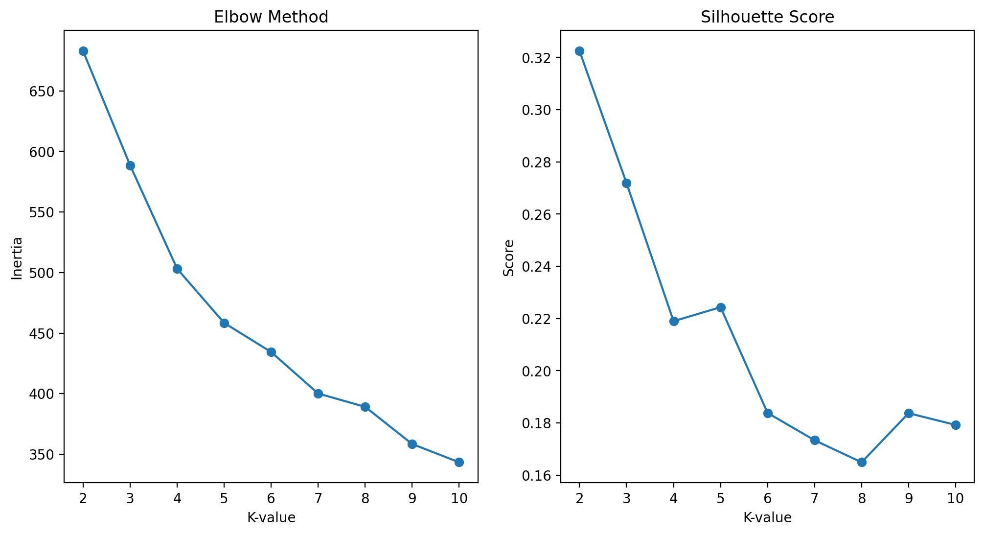
Based on the combined analysis of inertia and silhouette score, there is no standout optimal value of K. Instead, the results suggest a weak but consistent clustering within the data.
The inertia curve shows a steady decrease with k, where the rate of improvement slightly diminishes after k = 5 and again after k = 7, indicating diminishing returns in cluster compactness.
The silhouette score peaks at k = 2, but this is an oversimplification and not a meaning result in the context of defining midfielder archetypes in football. There is a local maxima at k = 5, beyond which the silhoeutte score becomes relatively stable in a low range (0.17-0.19), indicating weak cluster separation. This suggests that while some clusetering sturcture exists, it is not well defined, which is a refelction of how different player archetypes exist on a continuum and each share specific traits.
Given the absence of a single distinct optimal k-value, a stability analysis is conducted over k = 5, 6, and 7, corresponding to a region of diminishing returns in inertia, relatively stable silhouette scores, and strong football interpretability.
Clustering Results
| Metric | Cluster 0 | Cluster 1 | Cluster 2 | Cluster 3 | Cluster 4 |
|---|---|---|---|---|---|
| Progression | -0.25 | -0.46 | +0.33 | +1.23 | +0.28 |
| Creativity | -0.18 | -0.60 | +0.57 | +1.73 | +0.05 |
| Defensive | -0.02 | +0.31 | -0.44 | -0.41 | -0.01 |
| Goal Threat | +1.25 | -0.51 | +0.20 | +0.98 | -0.37 |
| Possession | -0.49 | -0.25 | -0.35 | +0.97 | +0.90 |
Table 2.1: Shows the average Z-scores for each of the five categories for k = 5 clusters.
| Metric | Cluster 0 | Cluster 1 | Cluster 2 | Cluster 3 | Cluster 4 | Cluster 5 |
|---|---|---|---|---|---|---|
| Progression | -0.21 | -0.53 | +0.33 | +1.60 | +0.74 | +0.02 |
| Creativity | -0.07 | -0.66 | +0.64 | +2.14 | +0.58 | -0.21 |
| Defensive | -0.01 | +0.27 | -0.45 | -0.61 | -0.07 | +0.17 |
| Goal Threat | +1.30 | -0.53 | +0.23 | +0.96 | +0.23 | -0.46 |
| Possession | -0.41 | -0.40 | -0.35 | +0.88 | +1.43 | +0.50 |
Table 2.2: Shows the average Z-scores for each of the five categories for k = 6 clusters.
| Metric | Cluster 0 | Cluster 1 | Cluster 2 | Cluster 3 | Cluster 4 | Cluster 5 | Cluster 6 |
|---|---|---|---|---|---|---|---|
| Progression | -0.22 | -0.34 | +0.44 | +1.63 | +0.68 | +0.17 | -0.50 |
| Creativity | -0.15 | -0.48 | +0.78 | +2.20 | +0.73 | -0.07 | -0.61 |
| Defensive | -0.16 | +0.82 | -0.43 | -0.55 | +0.02 | -0.13 | -0.18 |
| Goal Threat | +1.34 | -0.35 | +0.39 | +0.90 | +0.25 | -0.44 | -0.53 |
| Possession | -0.52 | -0.13 | -0.30 | +0.95 | +1.62 | +0.63 | -0.41 |
Table 2.3: Shows the average Z-scores for each of the five categories for k = 7 clusters.
Analysis
Beginning with k = 5, the following distinct archetypes emerge:
- Cluster 0 - Box Crashers - This cluster is characterised by a very high Goal Threat score (1.25) and below-average scores in all other categories. This suggests players whose primary contribution comes in advanced attacking situations, particularly through late runs into the box or by occupying dangerous positions. As a result, this group includes both physically dominant players who attack aerial balls (e.g. Scott McTominay and Mikel Merino) and more technical players who find space in the box (e.g. Curtis Jones). This highlights that similar statistical outputs can arise from different underlying playstyles.
- Cluster 1 - Anchors - This cluster is defined by the only above-average Defensive score (0.31), so broadly captures deeper-lying players with high defensive involvement, from aerially dominant players to excellent 1v1 defenders. Since this is the only cluster that encompasses the defensive score, there is considerable variation in the profiles observed. For example, players like Amadou Onana combine defensive strength with physical goal threat, while others such as Zubimendi contribute more in build-up. This suggests that defensive contribution alone is not sufficient to fully distinguish midfield roles.
- Cluster 2 - Progressive Creators - This cluster combines good Creativity (0.57) and Progression (0.33) with relatively low Possession involvement (-0.35). These players appear to operate as dynamic, risk-taking midfielders who drive play forward and attempt to create chances, rather than controlling tempo. Their lower Possession score may reflect a tendency to attempt higher-risk actions, resulting in less stable ball retention. This profile aligns with modern “advanced 8s” or secondary creators, such as Bruno Guimarães and Adam Wharton.
- Cluster 3 - Elite Players - This cluster exhibits elite levels of play across all attacking categories. Rather than representing a single tactical role, this group appears to capture the most influential attacking midfielders in the dataset. The presence of players such as James Maddison and Pedri illustrates this: while both are highly effective, their stylistic roles differ significantly. This suggests that the cluster may be separating overall quality and influence rather than a clearly defined positional archetype.
- Cluster 4 - Deep-Lying Playmakers - This cluster is defined by an excellent Possession score (0.90), representing players who are heavily involved in ball circulation and build-up play. These midfielders are likely responsible for maintaining possession and controlling tempo, often operating deeper on the pitch. However, variation still exists within the cluster: while players like Frenkie de Jong exemplify a classic deep-lying playmaker, others such as Eduardo Camavinga combine this with greater physicality and dynamism. This again highlights the fluidity of modern midfield roles.
Overall, the k = 5 clustering reveals several intuitive midfielder archetypes, including attacking playmakers, defensive specialists, and possession-focused players. However, significant variation exists within each group, and in some cases (notably Cluster 3), the model appears to separate players based on overall quality and influence rather than strictly defined roles. This demonstrates that traditional positional labels (CMs, CDMs, CAMs) are insufficient to fully describe the diversity of modern midfield profiles.
Moving to k = 6, the overall structure of the clustering remains largely consistent with k = 5. Clusters 0, 1 and 2 remain relatively stable, still identifiable as the Box Crashers, Anchors and Progressive Creators. The largest change at k = 6 is the refinement of the possession-based roles, rather than the emergence of entirely new archetypes.
- Cluster 3 - Playmakers - While this cluster continues to capture the most elite players, it becomes more extreme, particularly in Progression (1.23 to 1.60) and Creativity (1.73 to 2.14), so we can roughly define this cluster as the Playmakers. Despite their statistical separation, there is still considerable variation in profiles within this cluster (e.g. Pedri and Maddison). This reinforces the idea that the model still struggles to differentiate between quality and tactical role.
- Cluster 4 - Controllers - A new cluster that emerged from the Elite Attacking Playmakers, defined by an elite Possession score (1.43). These players are heavily involved in dictating tempo and controlling build-up play. The grouping of players such as İlkay Gündoğan, Vitinha and Frenkie de Jong reflects a more coherent and intuitive archetype of high-level midfield controllers.
- Cluster 5 - Supporting Midfielders - This cluster largely emerges from the previous Deep-Lying Playmakers at k = 5, separated from what can now be seen as the elite Controllers in Cluster 4. While still above average in Possession (0.51), these players contribute less in Progression (0.02) and Creativity (-0.21), but show higher defensive involvement (0.17). This suggests a role focused on maintaining structure and supporting play rather than controlling it. A good example of this is the reclassification of Eduardo Camavinga into this cluster, which aligns with the intuitive sense of his previously discussed misidentification at k = 5.
Overall, the transition to k = 6 does not introduce fundamentally new midfielder roles, but instead provides greater granularity within existing archetypes, particularly by separating high-level Controllers from more supportive possession players. However, the issues observed at k = 5 remain: certain clusters, particularly Cluster 3, appear to reflect player quality and influence rather than distinct tactical roles, alongside high variation in player profiles within clusters. This indicates that while increasing k improves detail, it does not fully resolve the overlap between role and quality within the dataset.
At k = 7, once again the overall structure of the clustering remains consistent, with no fundamentally new archetypes emerging. As expected, the additional cluster leads to further fragmentation of existing archetypes, the most notable of which is the emergence of a distinctive defensive specialist cluster.
- Cluster 1 - Ball-Winners - Compared to k = 5 and k = 6, this cluster now provides a much cleaner identification of players whose primary role is to break up play and win duels, as reflected in the elite Defensive score (0.82). However, while this cluster isolates elite defensive contributors more effectively, there remains variation in secondary attributes (e.g. Zubimendi vs Onana), just as there was at k = 5 and k = 6.
- Cluster 4 - Controllers - This cluster represents a refinement of the Controllers identified at k = 6, with an even more extreme Possession score (1.62). It continues to group the likes of Vitinha and Frenkie de Jong, meaning the less involved creators have been split into a separate cluster.
- Cluster 5 - Recyclers - Similar to the Supporting Midfielders archetype at k = 6, this cluster is characterised by solid Possession involvement (0.63), but limited contribution in other areas, alongside slightly reduced defensive activity (-0.13). This profile aligns with players who prioritise safe ball circulation and structural stability, rather than directly influencing attacking play, such as Marc Casadó.
- Cluster 6 - Low-Impact Players - This cluster is defined by below-average scores across all categories, suggesting players with relatively low statistical involvement within their teams. Unlike other clusters, this does not represent a clear tactical archetype, but rather a residual grouping resulting from increased model complexity. Alongside the Attacking Playmakers (Cluster 3), this further highlights that the model is partially capturing quality rather than purely distinct player roles.
Overall, increasing to k = 7 provides limited additional insight compared to k = 6. While it does separate the elite defensive players, it introduces a residual cluster of low-involvement players that lacks tactical meaning. This suggests that the added complexity does not meaningfully enhance the interpretability of the clustering and instead reinforces the limitation that the model struggles to fully separate player role from overall influence.
Evaluation
Standard Deviations
| Metric | k = 3 | k = 5 | k = 6 | k = 7 |
|---|---|---|---|---|
| Progression | 0.52 | 0.65 | 0.76 | 0.74 |
| Creativity | 0.63 | 0.90 | 0.98 | 0.98 |
| Defensive | 0.37 | 0.31 | 0.35 | 0.44 |
| Goal Threat | 0.78 | 0.79 | 0.74 | 0.72 |
| Possession | 0.71 | 0.72 | 0.78 | 0.81 |
Table 3: Shows the standard deviation in the mean category score for all clustering results.
To quantify how well differentiated the clusters were at each level, we calculated the mean score for each of the five feature categories within each cluster and then calculate the standard deviation across the cluster means, as seen above. A high standard deviation for a particular category, such as Progression, indicates greater variation between the cluster means and therefore stronger differentiation in that aspect of midfield play. A low standard deviation suggests that the cluster means are more similar, indicating less differentiation between clusters in that category. We can use this measure to support our evaluation of each k-value.
At k = 3, the clusters broadly resemble the traditional roles of Central Midfielders, Defensive Midfielders and Attacking Midfielders, but demonstrate significant overlap and a lack of granularity. This is supported by relatively low variation in Progression (0.52), Creativity (0.63) and Defensive Contribution (0.37), demonstrating that the three-role model does not produce strongly differentiated profiles across these dimensions.
At k = 5, there is clear improvement. Variation increases across key dimensions, particularly Progression (0.65) and Creativity (0.90), leading to five distinct and interpretable archetypes: Box Crashers, Anchors, Progressive Creators, Elite Players and Deep-Lying Playmakers. However, all players with a strong defensive score are grouped into one broad cluster, encompassing players with vastly differing profiles. Another issue that arises is that the model struggles to differentiate quality from tactical role. This is seen in Cluster 3, the Elite Players, who have far above-average scores across all metrics, but comprise a set of players with varying tactical roles.
At k = 6, the introduction of the extra cluster helps to further differentiate the possession-based roles, with variation increasing significantly across Progression (0.76), Creativity (0.98) and Possession (0.78). The primary improvement comes from the separation of the highly influential Controllers from the secondary Supporting Midfielders. This provides a more nuanced view of midfield roles, but still shares the same limitations as k = 5, with defensively dominant midfielders grouped together and an even more extreme separation of the elite players, who are now redefined as the Playmakers.
At k = 7, although defensive specialists are more clearly isolated (Defensive variation = 0.44), the clustering becomes more fragmented. The introduction of the Low-Impact Players, defined by below-average scores across all categories, does not represent a meaningful tactical role, but rather reflects differences in overall player influence. This highlights a key limitation of the model: its tendency to partially capture player quality alongside tactical role.
Conclusion
The purpose of this analysis was to evaluate whether the traditional classification of midfielders into three roles (CMs, CDMs and CAMs) is sufficient to effectively describe roles within the modern game. Using K-Means clustering, we aimed to identify how many distinct player archetypes emerge from the data. While no single “perfect” value of k exists, we evaluated k = 5, k = 6 and k = 7 using both statistical measures and footballing interpretation.
Overall, k = 6 provided the best balance between statistical separation and interpretability. It captures meaningful distinctions between player roles, particularly within possession-based midfielders, while avoiding the fragmentation and reduced clarity observed at k = 7.
This led to the identification of six key midfielder archetypes:
- Box Crashers
- Anchors
- Progressive Creators
- Playmakers
- Controllers
- Supporting Midfielders
While this six-role framework provides a more detailed view than the traditional three-role model, it remains an oversimplification of reality. This is partly due to the way modern football is played: a midfielder does not have one task that they consistently perform. Modern midfielders do not operate within fixed roles; instead, their responsibilities are fluid and context-dependent. A single player may perform multiple functions within a match, adapting to the game state, team structure and tactical demands.
As a result, player archetypes should not be viewed as rigid classifications, but rather as overlapping profiles within a continuous spectrum of roles. This helps explain why, even with increased model complexity, some degree of overlap between clusters remains unavoidable. Rather than providing definitive labels for every midfielder, the clustering framework is therefore better viewed as a way of identifying the underlying dimensions and common profiles that characterise modern midfield play.