Match Report Generator
DATA ANALYSIS · DATA VISUALISATION
As a keen football fan, I have always found visual summaries of matches particularly useful, especially when I have not had the opportunity to watch the game. However, I often find myself searching across several different apps and websites to find momentum graphs, passing netoworks and shot maps just to get an idea of what happened during a match.
To solve this, I created my own match report generator, bringing all the visualisations I find most useful together in one place. The generator is built as a reusable Python engine, which extracts Sofascore match data and automatically produces a range of visualistations, including team average positons overlayed with player heatmaps, match momentum, cumulative xG, and team shot maps.
The generator works for any match, given the data is available on Sofascore, producing both static and interactive figures. This not only gives me a consistent way of reviewing matches, but also provides the foundations for the more detailed statistical and tactical breakdowns featured in the Match Reports section of this website.
Figures
The objective of the generator was to produce enough visuals to provide a summary of any given match. Using the data available from Sofascore the generator produces team average positions, overlayed with individual player heatmaps, match momentum, cumulative xG and team shot maps. The combination of these figures provides a detailed overview of the match and can be used for more detailed analysis.
Team Average Positions
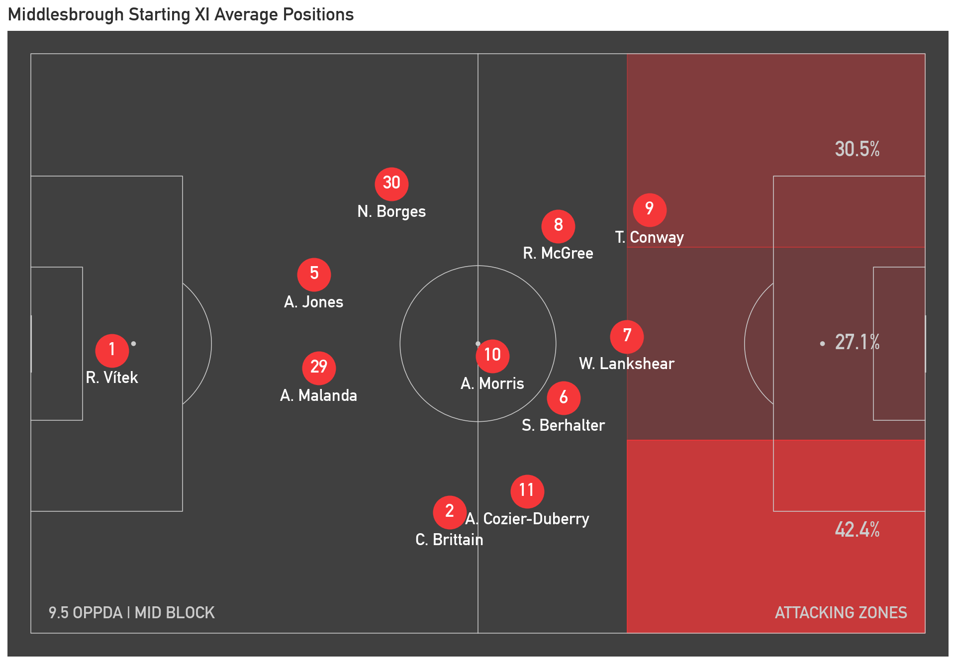
The first visual plots each teams's avearge positions using Sofascore's average position data. This data is the average coordinates of each palyers' touches, designating this as their "average position". The figure only visualises players in a team's starting XI since substitutes' average positions can appear unusual, due to a smaller sample size of touches, giving an inaccurate representation of a team's overall shape.
To enhance the figure, the non-interactive version also shows a team's tendancy to use each attacking zone. This is once again calculated using Sofascore's heatmap data, identifying touches in the attacking third and splitting these into the left, central and right zones based on the pitch coordinates. While the figure is biased towards showing a team' shape while in possession, the figure also shows a team's OPPDA (Opposition Passes Per Defensive Action). This metric is a rough estimate of how agressive a team are in winning the ball back when out of possession. A lower number, indicates a team gives their opposition less time on the ball pressing aggresively, while a higher number identifies a team that is content to sit deep and concede possession to their opposition. Using this metric it is possible to classify a team's out of possession approach as either a low-bloc, mid-block or high press.
The function to create the team's average player positions also provides the option to make the figure interactive. On top of the information provided by the static visuals, the interactive version provides the ability to hover over a player to display their heatmap as well of a selection of statistic to summarise thier game including: minutes played, touches, top speed and total distance covered. As well as the ability to toggle the attacking zones on and off to make the figure more interpretable, the interactive version provides a higher level of detail than the static version, making it a more suitable version for in depth analysis.
Below is an example of both the static and interactive average player positions for a Championship match between Middlesbrough and Norwich City.
Match Momentum
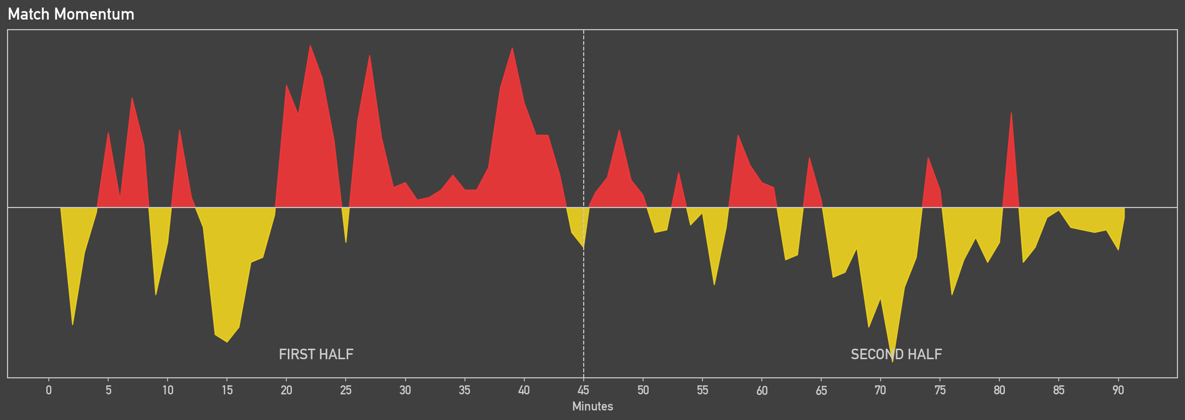
Match momentum is an intuative way to visualise how a match unfolded by showing which team was dominating play at any given minute in the match. It does this by calculating the possession value for each action on the pitch. As OPTA explains, the possession value measure the impact of an action on the pitch changing the probability of a team scoring in the next ten seconds. Then for any given minute, match momentum takes each team's most threatening situation, measured by possesssion value, and calculates the difference between these values to establish which team was more dominant. Thankfully, Sofascore provides match momentum data so that the engine just visualises the values.
Match momentum is a really useful metric to understand the narative of a game while very easily interpretable. Positve values show home team dominace while negative values show away team dominance and the taller the area, the more likely the team was to score in that moment. They can be used to undetstand how events like substitutions, tactical changes or breaks in play due to an injury can causes a shift in which team is dominating the match.
Below is an example of a match momentum figure for a Championship match between Middlesbrough and Norwich City.
Cumulative xG
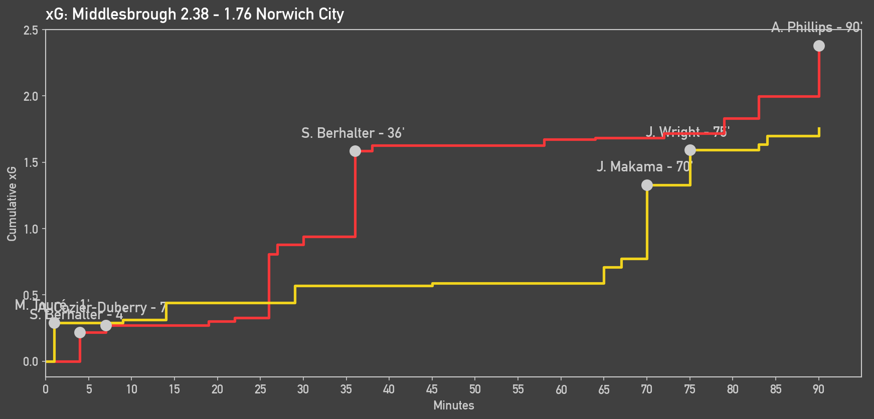
A cumulative xG graph is a way to demonstrate how frequently a team created chances over the match and what the quality of these chances was. Plotting the match time on the x-axis against total xG accumulated on the y-axis for each shot taken creates a stepped line. The more steps, the more shots a team had, while the higher an idivudual step is, the better quality chance it was. Rather than just stating a team's xG created over the match, the cumulative xG graph provides a more detialed overview of the rate and quality of chances. Paired with the match momentum, it provides an excellent explanation of a team's dominance in certain periods of a match.
Below is an example of a cumulative xG figure for a Championship match between Middlesbrough and Norwich City.
Shot Maps
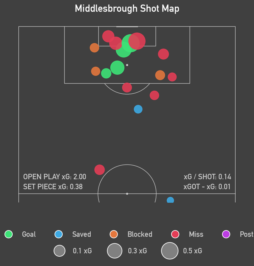
Shot maps are another way to explain what happened during a match by showing where chances came from and how good the chances were. The shot map function takes the coordinates of every shot in a match from Sofascore's shot data and plots it to visualise shot location. The quality of the chance is represented by the size of the point, scaled for xG, so the larger the point the better quality chance the shot was. As well as this, the shot points are colour-coded based on the outcome of the shot. To provide a little more detail about a team's overall chance creation, open play and set-piece xG are annotated on the figure, as well as xG / Shot to measure average chance quality and xGOT - xG to provide a metric of finishing quality.
The shot map also has the option to be drawn interactively. It displays all the same metrics as the static figure but upon hovering over a specific shot, it provides details of the player who took the shot, the minute, the xG, the xGOT, shot outcome, shot situation and the body part which took the shot. This provides extra detail to analyse a team's shooting tendancies.
Below is an example of a static and interactive shot map for Middlesbrough and Norwich City respectively, during a recent Championship match.
How It Works
The basis of the generator relies upon the ScraperFC package to obtain data from Sofascore. Given a match id, found in the Sofascore URL, the engine extracts the data required to generate tje report, saving it locally for further processing.
The data is automatically packaged into separate files. Team and player match stats, shot data, momentum data and average position coordinates are stored as CSV files, while heatmap data and player IDs are stored as pickle files due to their dictonary format. This creates a complete set of raw data that can then be accessed by the individual visualisation functions.
Each plotting function processes the raw data it requires independently using Pandas, cleaning and transforming it into a format suitable for visualisation. Some funcitons also calculate additioanl metrics, such as OPPDA and xG per Shot, while others perform transformations required for plotting, such as converting player coordinates between raw and display coordinate systems.
The generator is divided into five main functions, responsible for obtaining the data, producing avergae positions, match momentum, cumulative xg and shot maps. This modular structure means that individual figures can be generated independently rather than requiring the entire report to be produced each time. The functions are structured as follows:
scrape_data(match_id)plot_average_positions(team, team_colour, home_team, interactive = False)plot_momentum(home_colour, away_colour)plot_xg(home_team, home_colour, away_team, away_colour)plot_shot_maps(team, home_team = True, interactive = False)For the average positions and shot map functions, the engine supports both static and interactive outputs. Matplotlib and mplsoccer are used to produce static PNG figures, while Plotly is used for interactive HTML figures, allowing additional information to be displayed through hover interactions. Both types of figures are automatically saved to separate folders within the main file directory.
Technical Stack
| Area | Tools |
|---|---|
| Programming Language | Python |
| Data scraping | ScraperFC |
| Data processing | Pandas, NumPy |
| Static visualisation | Matplotlib, mplsoccer |
| Interactive visualisation | Plotly |
| Data source | Sofascore |
| Development | Jupyter |
| Version control | Github |
Challenges
In the intial versions of this project, there was only the option for static PNG figures. This was a fairly straight forward process, taking the data from Sofascore, cleaning with Pandas and plotting with matplotlib. The main challenge at this stage was the coordinate system compatability when plotting the shot map. The shot data from Sofascore used a 0-100 coordinate system, where the x-axis ran from a team's own goal to the opposing team's goal and the y-axis ran from the right flank to the left flank. However, for the shot map I wanted to plot a vertical, half pitch which did not align with the coordinates from the shot data. After investigating the coordinate system that mplsoccer's pitch was using, the raw coordinates required a transformation before plotting:
The main challenges arose in later versions of this project as I introduced interactive versions of the average positions and shot map figures. These figures were created using Plotly, which does not provide the same fotbball pitch plotting functionality as mplsoccer. I therefore had to create a blank plotly figure and write a helper function to manually draw each of the standard football pitch markings onto the figure. This had to be implemented twice, once for the full pitch used by the average positions figure and once for the vertically orientated half-pitch used for the shot map.
These manually constructed pitches also introduced a new challenge with the coordinate system. As previously mentioned, the raw data used a 0-100 coordinate system, meaning that both axes had the same numerical range. Directly plotting these coordinates would not correspond to the proportions of a standard football pitch. I therefore defined the pitch using the standard dimensiosn for a football pitch , 105x68, and transformed the coordinates accordingly.
For the average positions, this required a simple rescaling:
Whereas, for the shot map, which was plotted on the vertically orientated pitch, the raw coordinates needed to be reoriented by swapping the axes and reversing the vertical coordinates:
Future Improvements
Overall I am happy with what I have been able to achieve with this project. I have built a reusable match report generator that helps to interpret and analyse football matches. The figures the generated by the engine are easy to interpret and provide a detailed overview of a match, particuarly through the additional information provided by the interactive figures. However, there are still improvements I would like to make to this project.
The team average position figures are useful for understand the areas of the pitch in which players operate and can reveal underlying tactical structures that may not be apparent when a formation is labeled on paper. However, they provide limited information about a team's tendancies in possesion. To address this I would like to overlay passing networks on top of the average positions. This would provide greater insight into how teams build up in possession, demonstrate which players are central to their team's tactics and highlight the relationships between different players. To achieve this I would need access to match event-level data, containing detailed information individual passes, which is unfortunately not freely available through current data sources.
Another improvement I would like to make is to the match momentum figure. The current visualisation does a fantastic job at providing an intuative representation of which team controlled different periods of a match. However, by annotating specifc events on the timeline, such as substitutions, tactical changes, yellow cards and red cards, it would provide better explanation for swings in momentum. While this data is publically available, ScraperFC does not provide access to these events on Sofascore. One solution would be to manually add these events to a CSV file and annotate them on the momentum graph. However, this would ruin the reusability of the engine since it would need to be repeated manually for every match. A longer-term solution would be to identify a data source that provides information about match events and integrate it into the existing pipeline.
This project is still a work in progress as I seek to find additional data to enhance the figures but has been extremely useful for my understanding and analysis of football matches. If you would like to generate match reports for yourself, you can find the source code on GitHub.